Commercial catfish farming is a production business — it converts feed into fish biomass at a measurable rate, over a measurable period, producing a measurable output that sells at a measurable price. Every element of this conversion is quantifiable, and the quantities — feed consumed, biomass gained, time elapsed, population remaining — are the data that management decisions must be based on to be effective.
The farm manager who weighs fish monthly, tracks cumulative feed delivered, counts population through the grow-out period, and calculates FCR and daily growth rate from these measurements is managing with evidence. They know whether growth is on schedule three months before harvest. They know whether FCR is deteriorating two months before the financial consequences become visible. They know whether a mortality event has reduced the production population enough to warrant reducing the daily ration — preventing the overfeeding and water quality deterioration that following the original feeding rate would cause.
The farm manager who does not weigh fish routinely, does not track feed by pen or tank, and estimates growth and mortality from casual observation is managing with impression — and impressions are consistently less accurate than measurements. Studies of farmer production estimates versus measured production outcomes consistently find that farmers without systematic records overestimate fish size by 15–25%, underestimate mortality by 30–50%, and miscalculate FCR by margins that make production economics impossible to accurately assess. The financial consequences of these estimation errors accumulate invisibly through each production cycle and are only fully visible at the end-of-cycle financial reconciliation.
This guide provides the complete routine monitoring protocol for commercial catfish production — the sampling methods, population estimation techniques, growth calculation tools, and the specific management decisions that accurate monitoring data enables.
Sampling for Weight — Frequency, Method, and Sample Size
Why Monthly Weighing Is the Minimum Acceptable Frequency
Growth rate in African catfish is not uniform across the production cycle — it peaks in the early grow-out period (when fish are small and their tissue deposition rate per unit of body weight is highest), declines progressively as fish grow larger (as the maintenance energy requirement represents a larger fraction of total energy intake), and varies with temperature, feed rate, health status, and stocking density.
A feeding rate that is correctly calibrated to the fish’s biomass in Month 1 of grow-out is significantly incorrect by Month 3 — the biomass has roughly doubled (from initial stocking to approximately 50–100 g at typical growth rates), while the feeding rate calculated from Month 1 biomass has not changed. The fish are being underfed relative to their current appetite and growth potential, limiting growth rate and wasting the genetic potential the broodstock selection program created.
Monthly weighing corrects this progressive drift between assumed and actual biomass — providing the current biomass data that recalibrates the daily ration, updates the FCR calculation, and allows the growth trajectory to be compared against the production schedule.
More frequent weighing (bi-weekly or weekly) is warranted:
- In larval and early fingerling stages (Days 1–30) where growth rate is so fast that a two-week-old feeding rate calculation may be 50% below the fish’s current biomass
- When disease events have caused unknown mortality that changes biomass independently of growth
- When FCR is above target and the diagnosis requires current biomass data
Less frequent weighing (bi-monthly) is acceptable only for:
- Late finishing stage (above 600 g) where the growth rate per unit of time is slower and the biomass-feeding rate relationship changes more gradually
- Operations with very stable, well-established production parameters where biomass estimation from previous growth data has been validated against actual weighing
Sampling Protocol
Sample size: For statistical reliability (sampling error below ±10% of true mean weight), the minimum sample size is:
- Tanks below 500 fish: sample 10% of the population (minimum 30 fish)
- Tanks of 500–2,000 fish: sample 50–80 fish
- Tanks or ponds above 2,000 fish: sample 80–100 fish
Random sampling: The sample must represent the full size range of fish in the population — not selectively capturing the fish that are easiest to net (which are typically the largest, most active individuals), which would produce an overestimate of average weight.
Achieving representative sampling in concrete tanks:
- Reduce tank water level to 30–40 cm depth — concentrating fish and improving netting efficiency
- Use a seine net drawn across the full tank width — this samples fish from the full tank area rather than the corners where easy netting is possible
- Transfer a random portion of netted fish to a measurement container
Achieving representative sampling in earthen ponds: Earthen pond sampling is more challenging because fish are distributed through a larger water volume and not all size classes are equally accessible to a surface net. Two approaches:
- Seine netting with a properly designed net (lead line on the bottom, float line at the surface) pulled across a section of the pond in multiple passes
- Cast net sampling at multiple locations across the pond, combining samples from different locations for a pooled measurement
Weighing procedure:
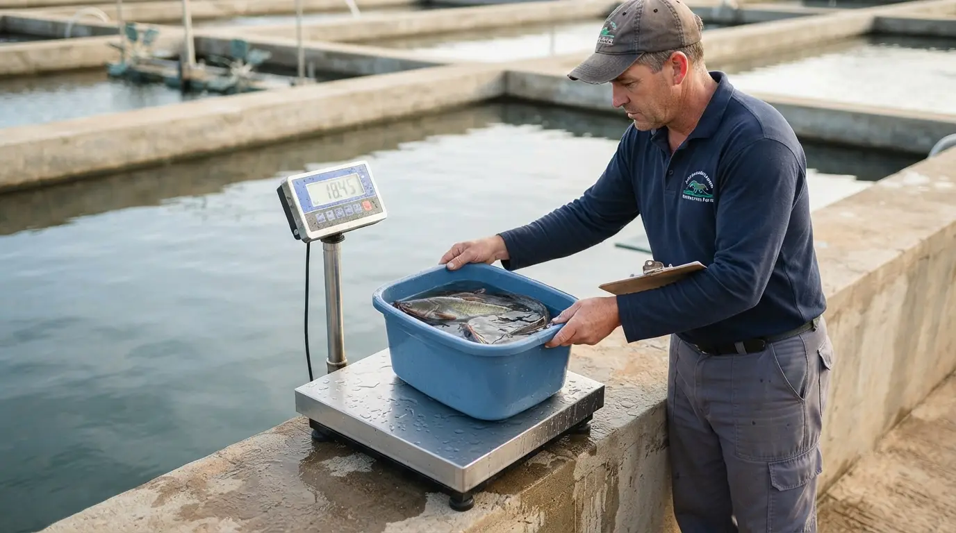
- Transfer sampled fish from the net to a bucket or container of tank water — minimize air exposure time
- Tare (zero) the weighing scale with an empty, water-wet container of the type that will hold the fish during weighing
- Count the fish into the weighing container, add sufficient water to submerge all fish, and record: (a) container + water + fish weight, (b) number of fish
- Calculate average individual weight: (Total weight – Container weight – Water weight) ÷ Number of fish
- Return fish to the tank promptly after weighing — minimize total handling time
Weighing accuracy targets:
- Scale capacity and precision: appropriate for the biomass being weighed (a 0.01 g precision analytical scale is inappropriate for 500 g fish; a 0.1 kg precision platform scale is appropriate for group weighing of grow-out fish)
- Tare verification before each weighing: verify the scale reads zero with the empty wet container before each group is weighed — scales drift under continuous use and in humid conditions
Recording Weight Data
For each weighing event, record:
| Field | Content |
|---|---|
| Date | Calendar date |
| Tank/pond ID | Production unit identifier |
| Sample size (number) | Number of fish weighed |
| Total sample weight (g or kg) | Gross weight minus container and water |
| Average individual weight (g) | Calculated from above |
| Minimum individual weight (g) | Smallest fish in the sample |
| Maximum individual weight (g) | Largest fish in the sample |
| Coefficient of variation (CV%) | Standard deviation ÷ mean × 100 — measures size uniformity |
| Estimated population count | Current estimated total fish in the unit |
| Estimated total biomass (kg) | Average weight × estimated count |
| Notes | Any observations: unusual behavior, lesions, feed response |
Population Counting and Mortality Tracking
Why Accurate Population Count Is Essential
The feeding rate calculation (daily ration = %BW/day × biomass) requires both the average fish weight AND the total fish count. An error in the population count produces proportional error in the calculated biomass and therefore in the daily ration:
If actual population is 450 fish but manager assumes 500 fish remain:
- Estimated biomass at 200 g average: 500 × 0.200 = 100 kg
- Actual biomass: 450 × 0.200 = 90 kg
- Feeding rate at 3% BW/day based on estimated biomass: 3.0 kg/day
- Correct feeding rate: 2.7 kg/day
- Overfeeding: 300 g/day = approximately 9 kg per month accumulated as uneaten feed
This overfeeding is not economically trivial — 9 kg of wasted feed at XAF 600/kg = XAF 5,400 per tank per month in direct waste, plus the water quality deterioration from organic loading that the wasted feed creates.
Methods for Population Estimation
Direct counting (the gold standard, practical only at harvest or complete tank drain):
When tanks are completely drained for harvest or cleaning, every fish is physically counted. This provides the definitive population count for each production unit — essential for FCR calculation (denominator is total weight gained by the actual fish present, not by the assumed population) and for mortality accounting.
Mortality accumulation tracking (continuous between harvests):
The most practical method for continuous population estimation — recording every fish that dies and subtracting from the initial stocking number:
Running population estimate = Initial stocked number − Cumulative mortality count
This method’s accuracy depends on complete mortality recording — every dead fish found during routine daily inspection must be counted and recorded. Missed mortalities (fish that die and are consumed by tank-mates before they are found, or that settle to pond bottom in earthen systems) cause progressive underestimation of actual mortality and overestimation of the remaining population.
Mitigation for missed mortalities: In earthen ponds where complete mortality collection is impractical, apply an estimated mortality discovery rate — if experience suggests that approximately 70% of dead fish are recovered before consumption or settling, multiply the recorded mortality count by 1.43 (= 1 ÷ 0.70) to estimate the actual total mortality. This estimated correction should be calibrated against actual counts at harvest.
Mark-recapture estimation (for large populations where counting is impractical):
The Lincoln-Peterson method for estimating large fish populations without counting every individual:
- Capture a sample of fish (N₁), mark them with a temporary or permanent marker (fin clip, paint mark, T-bar anchor tag), and return them to the population
- Allow 24–48 hours for the marked fish to redistribute randomly throughout the population
- Capture a second independent sample (N₂)
- Count the number of marked fish in the second sample (m)
- Calculate estimated total population: N = (N₁ × N₂) ÷ m
Example:
- First sample: 100 fish marked and returned
- Second sample: 80 fish captured, of which 16 are marked
- Estimated population = (100 × 80) ÷ 16 = 500 fish
This method requires that marked fish redistribute randomly — which requires at minimum 24 hours and is more reliable in well-mixed concrete tanks than in large earthen ponds where fish distribution may not be uniform.
The Daily Mortality Record
Every fish found dead in each production tank or pond should be recorded daily:
| Field | Content |
|---|---|
| Date | Calendar date |
| Tank/pond ID | Production unit |
| Mortalities found | Number of dead fish collected |
| Estimated average weight | Visual estimate of dead fish size |
| External signs | Brief description of any visible lesions or abnormalities |
| Probable cause | Best estimate: normal background, disease, water quality, predation |
| Action taken | Treatment initiated, water quality corrected, other response |
| Cumulative mortality | Running total for this production cycle |
| Cumulative mortality % | (Cumulative mortality ÷ Initial stock) × 100 |
The mortality rate as a monitoring trigger:
- Below 0.05% per day (grow-out): normal background — monitor, no intervention
- 0.05–0.1% per day: elevated — investigate water quality and health status; look for disease signs
- Above 0.1% per day: significant event — immediate investigation, consider treatment if disease identified
- Above 0.5% per day: emergency — all available management resources focused on diagnosis and response
Growth Calculation and Production Schedule Management
Key Growth Metrics
Average Daily Gain (ADG):
ADG (g/day) = (Current average weight − Previous average weight) ÷ Days between measurements
Example: Week 4 average weight: 45 g; Week 8 average weight: 95 g; Days between measurements: 28 days. ADG = (95 − 45) ÷ 28 = 1.79 g/day
Specific Growth Rate (SGR):
SGR is the daily growth rate expressed as a percentage of body weight — useful for comparing growth rate across different body size ranges:
SGR (%/day) = [(ln(W₂) − ln(W₁)) ÷ Days between measurements] × 100
Where W₁ = initial average weight, W₂ = final average weight, ln = natural logarithm
Example using the same data: SGR = [(ln(95) − ln(45)) ÷ 28] × 100 = [(4.554 − 3.807) ÷ 28] × 100 = [0.747 ÷ 28] × 100 = 2.67%/day
SGR values for commercial African catfish grow-out:
- Excellent: above 3.0%/day (small fish, 10–50 g)
- Good: 2.5–3.0%/day (50–150 g range)
- Acceptable: 2.0–2.5%/day (150–300 g range)
- Below average: 1.5–2.0%/day (300–500 g range)
- Poor: below 1.5%/day at any stage below 500 g (investigate cause)
Projecting Time to Market Weight
Once current average weight and current growth rate are established from routine monitoring data, time to market weight can be projected:
Simple linear projection (adequate for short remaining production periods):
Remaining days to harvest = (Target market weight − Current average weight) ÷ Current ADG
Example: Target market weight: 1,000 g Current average weight (Week 8): 95 g Current ADG: 1.79 g/day Remaining days = (1,000 − 95) ÷ 1.79 = 505 days
This projection is clearly unrealistic — it assumes the current ADG (appropriate for a 45–95 g fish) continues unchanged to 1 kg. Growth rate declines as fish grow larger, so linear projection from early-cycle ADG dramatically overestimates time to market weight.
Growth rate adjustment with body size:
For more accurate projections, apply the documented relationship between body size and growth rate in African catfish:
| Size Range | Expected ADG | Expected SGR |
|---|---|---|
| 10–50 g | 2.5–4.0 g/day | 3.0–4.5%/day |
| 50–150 g | 3.0–5.0 g/day | 2.5–3.5%/day |
| 150–300 g | 4.0–7.0 g/day | 2.0–3.0%/day |
| 300–600 g | 5.0–9.0 g/day | 1.5–2.5%/day |
| 600–1,000 g | 6.0–10.0 g/day | 1.0–2.0%/day |
Using size-specific ADG values to project forward through successive size intervals provides more accurate harvest date projections. For practical production planning purposes, the most reliable projection method is:
- Use the average SGR observed over the most recent monthly weighing interval
- Apply this SGR forward for 30-day intervals, recalculating projected weight at each interval
- Identify the 30-day interval in which projected weight crosses the market weight threshold
Tracking Growth Against Production Schedule
The production schedule — the planned date at which fish should reach market weight based on the stocking date, initial fingerling weight, and expected growth rate — is the baseline against which monthly growth monitoring data should be compared:
Growth schedule comparison table (example, 10 g fingerlings, 28°C, target 1 kg):
| Month | Expected Average Weight | Acceptable Minimum Weight | Management Action if Below Minimum |
|---|---|---|---|
| 0 (stocking) | 10 g | 8 g | — |
| 1 | 60–80 g | 45 g | Check water quality, feed rate, parasite load |
| 2 | 180–220 g | 130 g | Water quality investigation, health check |
| 3 | 380–450 g | 300 g | Disease investigation, feed quality review |
| 4 | 600–700 g | 500 g | Management review — all parameters |
| 5 | 900–1,050 g | 750 g | Harvest planning; market timing adjustment |
When measured growth falls below the acceptable minimum at any checkpoint, the monitoring data has provided a 30–60 day warning of a production schedule deviation — allowing corrective action before the delay becomes a harvest date problem that affects market commitments.
Size Uniformity Assessment and Management
Why Size Uniformity Matters Economically
A tank of catfish that has grown from uniform 10 g fingerlings to an average of 500 g at Month 4 could contain fish ranging from 200 g to 800 g — or fish tightly clustered around 450–550 g. Both populations have the same average weight, but their commercial and operational implications differ dramatically:
The non-uniform population:
- Partial harvests required — fish must be harvested in multiple events as different size classes reach market weight
- Ongoing cannibalism pressure from larger fish on smaller ones — continued mortality and size disparity
- Lower per-fish sale value for the small portion of the batch that must be sold below market weight
- Complex market logistics — small volumes harvested at different times rather than a single scheduled harvest event
The uniform population:
- Single harvest event at a predictable date — simplifying market planning and logistics
- No ongoing cannibalism after the early grow-out period where grading has maintained uniformity
- Consistent product presentation to buyers — all fish at or near target weight
- Higher total sale value from consistent premium market pricing
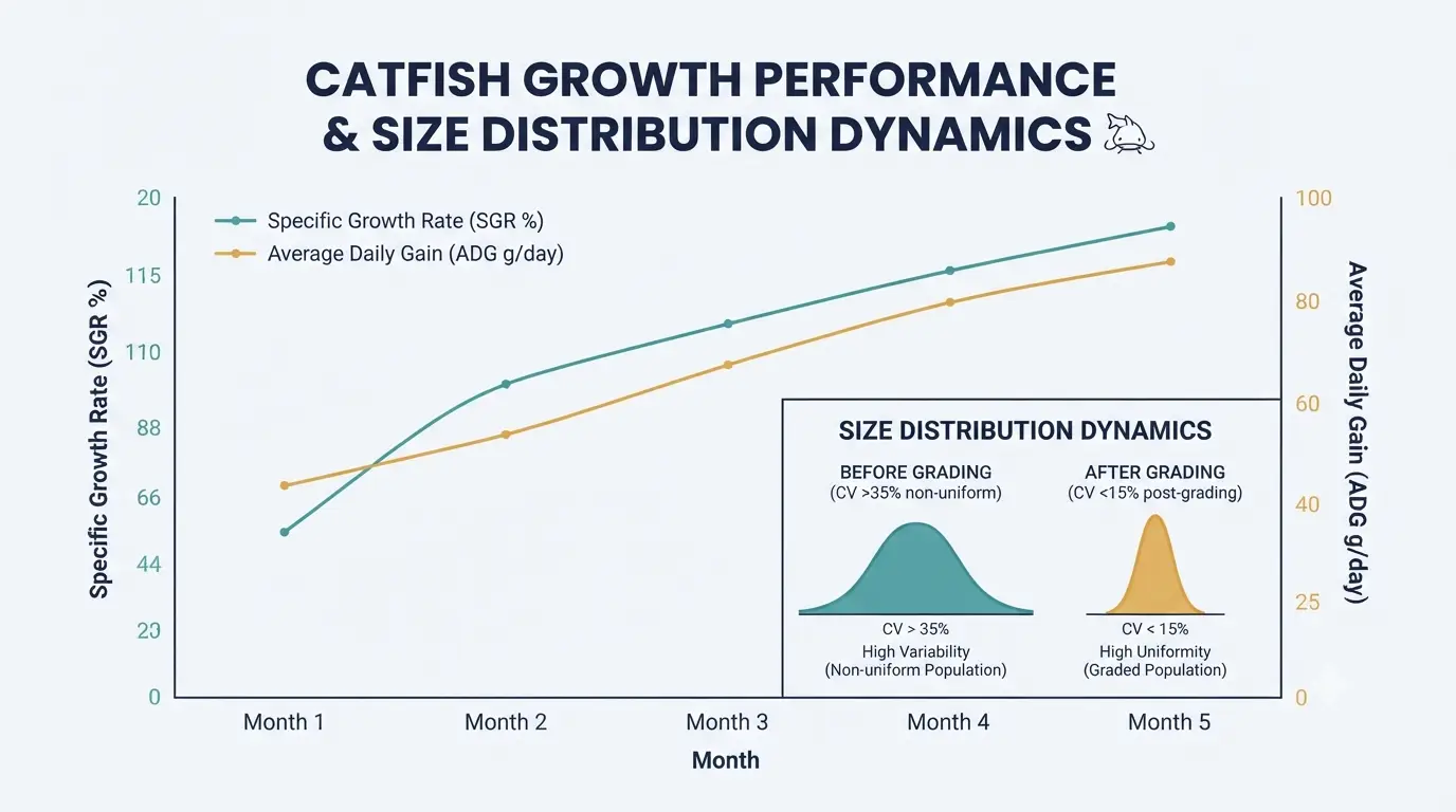
Measuring Size Uniformity — The Coefficient of Variation
The coefficient of variation (CV) is the standard statistical measure of size uniformity in a fish population:
CV (%) = (Standard deviation of individual weights ÷ Mean weight) × 100
Calculation from a sample:
- Measure individual weights for 30–50 fish from the sampling event
- Calculate mean weight: sum all weights ÷ number of fish
- Calculate standard deviation: the square root of the average squared deviation from the mean
- CV = (Standard deviation ÷ Mean) × 100
Interpretation:
| CV Range | Uniformity Assessment | Management Implication |
|---|---|---|
| Below 15% | Excellent uniformity | Single harvest possible; minimal size-related competition |
| 15–25% | Good uniformity | Single harvest possible with size sorting at harvest |
| 25–35% | Moderate non-uniformity | Consider grading before market weight to improve uniformity |
| 35–50% | Poor uniformity | Grade now; investigate cause; partial early harvests |
| Above 50% | Very poor uniformity | Emergency grading; active cannibalism investigation |
Maintaining Uniformity Through the Production Cycle
Sources of increasing size variation through the grow-out period:
Growth rate variation in a catfish population is inevitable — some individuals grow faster than others due to genetic variation in growth capacity, differential access to feed in competitive feeding situations, and the compounding effect of initial size variation from imperfect grading at stocking.
The key management insight is that size variation is self-amplifying without intervention: larger fish dominate feeding positions, consuming a disproportionate share of the ration, growing even faster while smaller fish receive proportionally less feed and grow more slowly. The gap between the largest and smallest fish in an ungraded population widens every month from stocking to harvest.
Grading during grow-out:
A mid-cycle grading event — separating the population by size into two or three groups that are then managed separately — interrupts the self-amplifying cycle. Each re-sorted group, now more uniform within itself, can be fed and managed optimally for its size range without the cross-group competition that drives the uniformity decline.
Practical mid-cycle grading protocol:
- Drain the tank to 30–40 cm water depth
- Seine net the population and transfer to a collection container
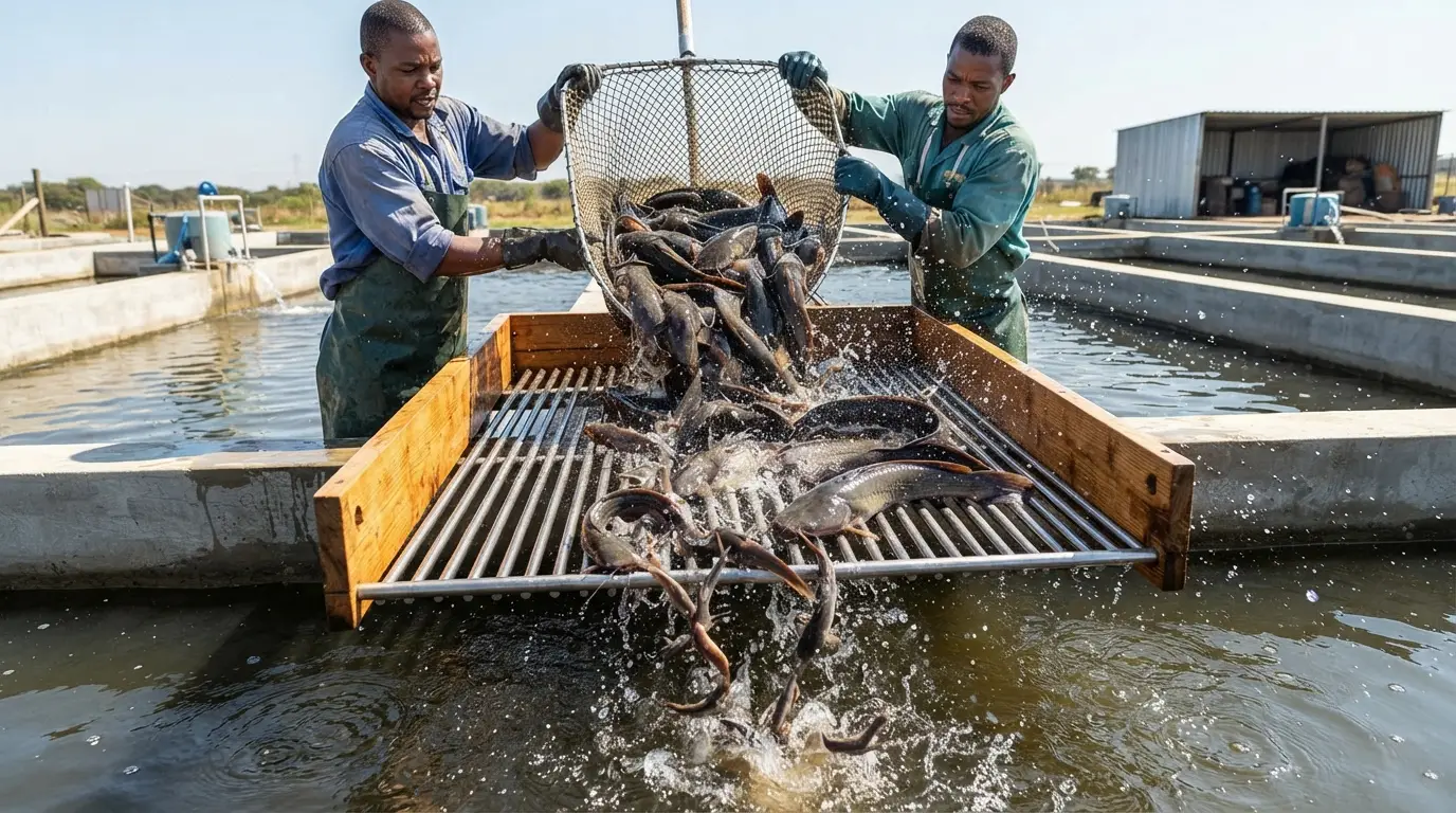
- Pass fish through a grading screen (a frame of parallel bars with adjustable spacing) — fish smaller than the bar spacing pass through to a “small” collection; fish larger remain on the screen as “large”
- Restock the large group in the original tank at the correct stocking density for their current size
- Restock the small group in a separate tank at appropriate density — providing separate management, including potentially a higher protein diet or longer production cycle
Integrating Growth Data With Production Management Decisions
The Monthly Management Review
Growth monitoring data generates the production management decision inputs that the formal monthly review should address:
Feeding rate update:
Using the current average weight (from monthly weighing) and current estimated population count (from cumulative mortality tracking):
- Calculate current estimated biomass: average weight × estimated count
- Apply the appropriate %BW/day feeding rate for the current average weight and water temperature
- Calculate the updated daily ration
- Update the daily feeding instruction for the tank — communicated clearly to feeding staff so the change is actually implemented
FCR update:
Using feed delivered since last weighing and biomass gain since last weighing:
- Total feed delivered (from feed delivery records): sum all feed weighed and delivered to the tank
- Biomass gain: (current average weight × current estimated population) − (previous average weight × previous estimated population, accounting for mortality)
- Monthly FCR = Total feed delivered ÷ Biomass gain
- Compare to target: investigate if above target using the diagnostic framework from the FCR article
Harvest date projection update:
Using the updated current average weight and the most recent growth rate (calculated from the current and previous weighing events):
- Calculate current ADG from the most recent weighing interval
- Project time to market weight using size-adjusted ADG as described in Part 3
- Compare projected harvest date to the market commitment date — if the projection shows a delay, identify and address the growth rate limitation causing the deviation
Stocking decision support:
The population counts from ongoing mortality tracking, combined with the growth trajectory projection, provides the data for the next stocking planning:
- When will the current tank be available (harvest date projection)?
- How many fish are projected to be harvested (current count minus projected additional mortality)?
- What fingerling volume should be ordered, and for what delivery date?
The Cumulative Production Report
Building the Production Record
Beyond the individual monthly snapshot, the cumulative record assembled from monthly monitoring data provides the longitudinal production view that management learning depends on:
Per production cycle summary (compiled at harvest):
| Parameter | Value | Calculation |
|---|---|---|
| Production unit | Tank/pond ID | — |
| Species and strain | — | From stocking record |
| Stocking date | — | From stocking record |
| Harvest date | — | Recorded at harvest |
| Production cycle length (days) | — | Harvest date − Stocking date |
| Initial stocking number | — | From stocking record |
| Initial average weight (g) | — | From Day 1 weighing |
| Final harvest number | — | Counted at harvest |
| Final average weight (g) | — | Weighed at harvest |
| Total mortality | — | Initial number − Final number |
| Mortality rate (%) | — | Total mortality ÷ Initial stocking × 100 |
| Total feed delivered (kg) | — | Sum of all recorded feed deliveries |
| Total weight gained (kg) | — | (Final weight × Final count) − (Initial weight × Initial count) + (Estimated dead fish weight) |
| FCR | — | Total feed ÷ Total weight gained |
| ADG (g/day) | — | (Final average weight − Initial average weight) ÷ Cycle length |
| Total harvest weight (kg) | — | Final average weight × Final count |
| Sale price per kg | — | From sales record |
| Gross revenue | — | Total harvest weight × Sale price |
| Feed cost | — | Total feed × Feed price per kg |
| Net margin | — | Gross revenue − All costs |
Using the Production Record for Continuous Improvement
The cumulative production record, maintained for every production cycle in every tank, provides the dataset that converts farm management from repetitive trial-and-error to systematic continuous improvement:
Year-on-year comparison: Is average FCR across all cycles in Year 2 better than Year 1? Which specific management changes between the years can explain the difference?
Tank comparison: Is Tank A consistently achieving better FCR than Tank B with equivalent stocking density and feed? The water quality parameters in each tank, the management practices of the staff responsible for each tank, and the feed delivery records provide the variables to investigate.
Seasonal pattern analysis: Is the production cycle started in October consistently achieving better growth rates than the cycle started in March? Temperature data confirms whether this is a temperature-driven growth rate difference or something else.
Disease event impact quantification: How much did the Aeromonas event in Tank C during Month 3 cost in terms of FCR deviation from the operation’s average? This quantification converts disease management from a veterinary cost center to a production economics calculation with measurable ROI for prevention investment.
Summary
Routine sampling, growth tracking, and population monitoring convert catfish farming from a process managed by impression to a production system managed by evidence. The monthly weight measurement, the daily mortality record, the cumulative feed delivery log, and the calculations that convert these records into growth rate, FCR, population estimates, and harvest date projections — together constitute the information system that allows the farm manager to make correct feeding, treatment, stocking, and marketing decisions based on what is actually happening in each tank rather than what appears to be happening from casual observation.
The investment in this monitoring system is modest — a scale, a mortality log, a weighing notebook, and the 30–60 minutes per week required to perform the measurements, complete the records, and calculate the key metrics. The return — early detection of growth deviations that allows corrective action before schedule impact, FCR calculations that identify the feed cost consequence of management decisions, and population estimates that correctly calibrate feeding rates and market planning — is the foundation of operational profitability that no amount of disease treatment, feed quality investment, or genetics improvement can provide without accurate production monitoring as its basis.
The final article in the catfish farming cluster covers the digital tools and software systems that make these monitoring and record-keeping functions more efficient and accessible for commercial catfish operations of any scale.